Past 40 km, design from measured span loss and check three limits in turn: attenuation, chromatic dispersion and, once amplifiers appear, optical signal-to-noise ratio.
01The connection brief
Beyond about 40 km a link stops being a cabling exercise and becomes an optical engineering exercise. This page is a planning concept for spans in the 80 to 120 km range and the design work they require. It is a reference method rather than an account of a delivered route, and it names no operator, route, country or result.
The brief is normally one span between two sites, over owned or leased fiber, carrying an aggregate that has outgrown a lower-rate link. What distinguishes it from a campus link is that three separate effects can each end the design: attenuation, chromatic dispersion, and, once amplifiers appear, optical signal-to-noise ratio. None of the three can be inferred from the headline reach on a datasheet.
02The design inputs
The single most important input is a measured loss figure for the span at the working wavelength, taken with a light source and power meter, together with an OTDR trace. A route length taken from a map is not a design input at this distance, because duct routing, slack loops and repair splices routinely add both length and loss.
Record the fiber type, since standard single-mode fiber and dispersion-shifted variants behave very differently at 1550 nm. Record the splice count and estimated splice loss, any leased segment with a contractual loss limit, and the position of any intermediate site where amplification could be housed. Record the required rate, the host platforms at both ends with their software releases, and whether the span carries one channel or several.

03The topology and optical path
A long span is usually a simple two-ended path, but its internals matter. Write out every element: transmit module, station jumper, station panel, outside plant cable, each splice enclosure, the far station panel, far jumper and receive module. An 80 km route frequently contains dozens of splices, and while each is small at about 0.1 dB, the total is not.
Decide early whether the span carries a single channel per fiber pair, a single-fiber BiDi arrangement, or several channels multiplexed onto one pair. Multiplexing adds the insertion loss of the multiplexer and demultiplexer at each end, which is a substantial and often overlooked addition to a budget that is already tight.
04Product families to evaluate
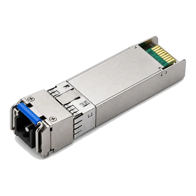
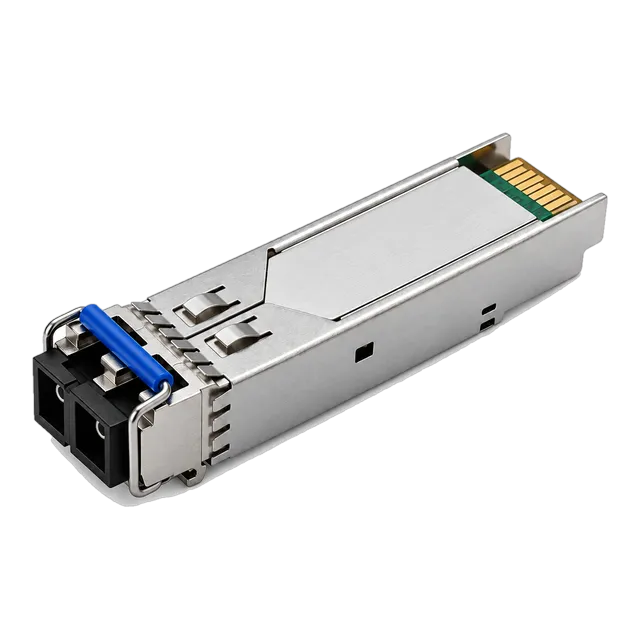
For 10 gigabit single-fiber spans the 10G SFP+ BiDi BX80 80km 1490/1550nm Simplex LC DDM APD module and the SFP-10G-BX100 10G BiDi 100km 1490/1550nm Simplex LC SMF module are the relevant families, both using the longer wavelengths where attenuation is lowest. At 2.5 gigabit, the 2.5G BiDi SFP-2.5G-BX120 Single-Fiber 1490/1550nm 120km module covers the longest single-fiber case, and at gigabit the 1.25G SFP Dual-Fiber LC DDM 1550nm 80km module applies.
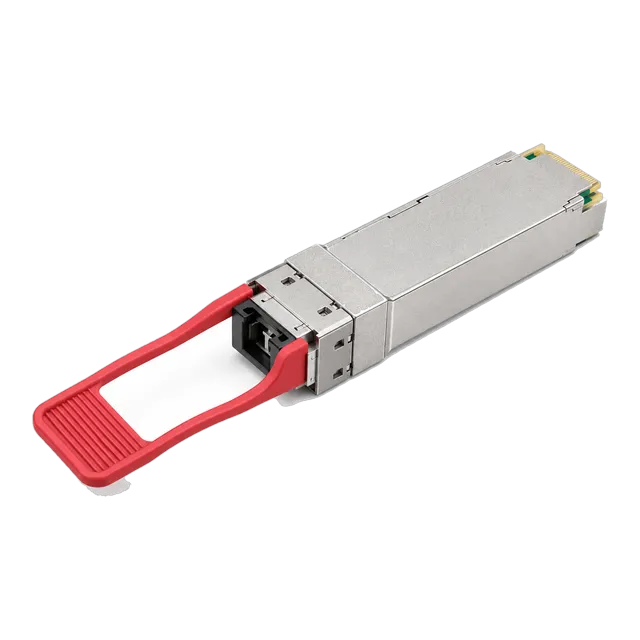
At higher rates the 25G SFP28 ZR 1310nm 80km module, the 40G QSFP+ ZR 1310nm 80km Single-Mode Duplex LC module and the 100G QSFP28 eZR4 100km LWDM4 Duplex LC module cover long spans, with the 40G QSFP+ CWDM4 1310nm 60km module for intermediate distances.
05Link budget and reach considerations
Start with attenuation. At 1550 nm plan on roughly 0.22 dB/km, so an 80 km span contributes about 18 dB before anything else. At 1310 nm the figure is roughly 0.35 dB/km, which is why long spans prefer the longer wavelength. Add mated connector pairs at 0.3 to 0.75 dB, splices at about 0.1 dB each, and any multiplexer insertion loss. Keep about 3 dB of unallocated margin.
Compare the total against the difference between minimum launch power and receiver sensitivity. Long-reach modules achieve their sensitivity with avalanche photodiode receivers, which buy several decibels over a PIN receiver but also have a lower maximum input power, so the overload point must be checked as carefully as the sensitivity.
06Dispersion and signal quality
Attenuation is only the first limit. Standard single-mode fiber has chromatic dispersion of roughly 17 picoseconds per nanometre per kilometre at 1550 nm, and that accumulates with distance. At 10 gigabit and above it produces a dispersion penalty that can close the eye even when received power is comfortable, which is why a datasheet quotes a dispersion tolerance as well as a power budget.
At 1310 nm dispersion is near zero on standard fiber, which is why several long-reach classes at 25, 40 and 100 gigabit use that region despite its higher attenuation. Where the calculation shows dispersion rather than power as the limit, the answers are a lower-dispersion wavelength plan, dispersion compensation, or a coherent transport system rather than a higher-power module.
07Environment, amplification and power
Station environments are usually conditioned, so commercial grade optics rated 0 to 70 degrees Celsius are normally appropriate, but long-reach modules dissipate more heat than short-reach ones and a densely populated line card should be checked rather than assumed.
If the budget does not close, amplification is the next step, and it changes the nature of the design. An optical amplifier adds noise as well as power, so the span then has to be assessed for optical signal-to-noise ratio rather than only for received power, and amplifier placement, gain and any need for gain flattening become part of the plan. Amplified designs also need a safety review, because the launch powers involved demand proper handling procedures on open connectors.
08Validation and acceptance
Long spans deserve measurement before purchase, not after. Obtain the end-to-end loss at the working wavelength and a full OTDR trace in both directions, and reconcile the two, since a one-way trace hides events near the far end.
At commissioning, read digital diagnostics at both ends and confirm received power sits comfortably inside the window between sensitivity and overload. Then look at error behaviour over time rather than at a snapshot, because dispersion-limited and marginal-power links often pass a brief test and fail across a temperature cycle. Run an extended soak covering at least one full day-night cycle, and record loss, DDM values and error counters as the baseline for the span.
09Procurement and BOM
The BOM for a long span is short but each line carries assumptions that should be written next to it. It holds two matched transceivers, the station jumpers, any multiplexer pair, any fixed attenuators from the budget calculation, and amplification hardware where the design needs it.
BiDi spans use two different part numbers in matched quantities. Attenuators belong in the initial BOM whenever the calculation suggests the receiver could be overloaded, particularly where a 100 or 120 km class module is being used on a shorter span. Coding is confirmed per host platform and recorded alongside the optical specification. Spares policy for long-span modules is usually set per span rather than as a blanket percentage, because a single span failure removes the whole path.
10Common mistakes
The most common error is designing from route length on a map rather than from a measured loss figure, which understates a real span by a wide and unpredictable margin. The second is checking attenuation and ignoring chromatic dispersion, so a link with healthy received power still errors.
The third is overlooking the overload point of an avalanche photodiode receiver and installing a 100 km class module on a 30 km span. The fourth is forgetting multiplexer insertion loss when several channels are combined onto one pair. The fifth is adding an amplifier to fix a power shortfall without then assessing optical signal-to-noise ratio, which simply substitutes one limit for another.
11Next step
Before selecting parts, obtain the span measurements: end-to-end loss at the intended wavelength, a bidirectional OTDR trace, the splice count and the fiber type. Add the required rate, the host platforms with their software releases, and any intermediate site available for equipment.
Then add candidate 10G SFP+, 2.5G SFP and 100G QSFP28 long-reach items to an inquiry list, noting the calculated budget and the dispersion check alongside each. The project worksheet provides blank fields for the same inputs. This page is a planning concept rather than a delivered route design, so every figure quoted here is a method to apply to real measurements rather than a result that can be reused on another span without recalculation.
12Design inputs to document
| Design input | What to record |
|---|---|
| Measured span loss | End-to-end loss at the working wavelength, not a map distance. |
| OTDR trace | Bidirectional trace with splice positions and individual losses. |
| Fiber type | Standard single-mode or a dispersion-shifted variant. |
| Splice and connector count | Total mated pairs and fusion splices across the span. |
| Required rate and channels | Single channel, BiDi on one strand, or multiplexed channels. |
| Dispersion tolerance | Datasheet figure for the candidate module against the span. |
| Intermediate sites | Any location available for amplification or regeneration. |
| Host platforms | Models and software releases at both ends, for coding confirmation. |
13Planning bill of materials
| Item | Configuration | Quantity |
|---|---|---|
| 10G SFP+ BiDi 80 km transceiver | 1490/1550 nm, simplex LC, APD receiver, DDM | 2 per span, matched pair |
| 10G SFP+ BiDi 100 km transceiver | 1490/1550 nm, simplex LC, single-mode, long-reach class | 2 per span, matched pair |
| 2.5G BiDi 120 km transceiver | 1490/1550 nm, simplex LC, single-mode, DDM | 2 per lower-rate span, matched pair |
| 100G QSFP28 eZR4 transceiver | LWDM4 in the 1310 nm region, duplex LC, 100 km class | 2 per high-rate span |
| Fixed optical attenuator | Value from the budget calculation, single-mode | To specify where overload is predicted |
| Station patch cords | Simplex or duplex to match the module and panel | 2 per span |
Planning quantities only. The final bill of materials is confirmed with your quotation.
14Frequently asked questions
Why do long spans use 1550 nm rather than 1310 nm?
Because attenuation is lower: roughly 0.22 dB/km against roughly 0.35 dB/km. Over 80 km that difference is about 10 dB, which is often the difference between a link that closes and one that does not. The trade-off is chromatic dispersion, which is near zero at 1310 nm on standard fiber and around 17 picoseconds per nanometre per kilometre at 1550 nm.
What does an APD receiver change in the design?
An avalanche photodiode gains several decibels of sensitivity over a PIN receiver, which is what makes 80 to 120 km classes practical. It also has a lower maximum input power, so the overload point becomes a real constraint. Check both ends of the window, and plan a fixed attenuator if a long-reach module will be used on a shorter span.
Can attenuation alone decide a long-haul design?
No. A span can have ample received power and still error because accumulated chromatic dispersion has closed the eye. Datasheets quote a dispersion tolerance alongside the power budget for exactly this reason. Check the span against both, and if dispersion is the binding limit, the answer is a wavelength or compensation change rather than more transmit power.
When should amplification be considered?
When the calculated budget does not close and the route cannot be shortened or its connections reduced. Adding an amplifier changes the assessment: the span then has to be evaluated for optical signal-to-noise ratio as well as for received power, and amplifier placement and gain become design parameters. It also raises launch powers enough to require careful handling procedures.
Technical review note: confirm model-specific specifications with the product datasheet and the intended host documentation. Product images and application photographs are illustrative.
Discuss this with our team